Adding virtual power to your Tacx T2600 workout using Python

In previous post 'Adding virtual power to tcx for Tacx' I talked about adding virtual power to your trainer workout. Today I made a Github repository with a Python program for doing that: vpower

What is needed to be able to add power ? First, you must record your speed during the workout. The power is specifically for the Tacx Blue Motion T2600. This model is not for sale anymore, but the Tacx Blue Motion 2650 is:

The lever for the manual resistance control must remain on the same position during the workout. I leave mine in position 5 and use my gears to alter the workload during the workout.

I use my Garmin 810 for recording but any cycling computer will work probably as well. The result from my Garmin 810 is a FIT file that I normally submit to Strava. If you want to add virtual power, you must do following steps before submitting to Strava:

1. Obtain a TCX file with speed during the workout: In case of a Garmin, I convert the FIT file of my workout to TCX (I use Garmin Training Center for that, but unfortunately Garmin does not offer it anymore for download).
2. Process the TCX file with the vpower.py program from the vpower repository. The result is an altered TCX file with power included. The added power element are derived from the speed you were riding at a certain moment during your workout. It is assumed that you did not altered the lever for the manual resistance control during the workout. Since the lever of the Tacx T2600 is purely mechanical, it can not be recorded by your cycling computer during the workout.
3. Upload the altered TCX file to Strava.

Here's an example workout on the Tacx Blue Motion T2600 with virtual power added:

Why do I use TCX and not GPX? GPX has no extensions for power at this moment.

The linear formula to determine power from speed is based on following drawing:

Suppose that your lever for manual resistance control is at position 5 and your riding at 30km/h, your power is then a little less then 250 Watt.

Kaggle competitions

Since a few weeks, I'm participating in Kaggle data science competitions. First I entered the Titanic survival competition and now I'm trying to predict sales for the German Rossman stores. I wrote a jupiter notebook with some basic exploration. You can view the notebook on github or get an even nicer view on NBviewer NBviewer.
Enjoy,
Lode

Calculating Heart Rate zone based on Lactate Threshold Heart Rate

I already investigated the issue of setting heart rate zones in blogpost "Setting Strava heart rate zones based on Lactate threshold heart rate (LTHR)". In the article "HOW TO FIND YOUR HEART RATE ZONES" all zones are defined along with the protocol to determine your lacatate threshold yourself:

• Z1 < 81% of LTHR 
• Z2  81% - 89% of LTHR
• Z3 90% - 93% of LTHR
• Z4 94%-99% of LTHR
• Z5a 100%-102% of LTHR
• Z5b 103%-106% of LTHR
• Z5c > 106% of LTHR

The definition of the zones correspond to those found in Joe Friel's book "The cyclist trainings bible" at page 37 Table 4.5.

Based on a LTHR of 175bpm my zones would be:

• Z1 Endurance: < 141 bpm
• Z2 Moderate: 142 - 156 bpm
• Z3 Tempo: 157 - 163 bpm
• Z4 Threshold: 164 - 173 bpm
• Z5a:  175 - 179 bpm
• Z5b: 180 - 185 bpm
• Z5c: 186 - 187 bpm

Parsing Strava GPX file with python minidom

GPX is more and more becoming the lingua franca for storing cycling rides. Basically it is a list of points, called track points, with satellite positions (latitude and longitude) decorated with extra information (elevation, heartrate, cadence, power or temperature). A track (<trk>), has one or more segments (<trkseg>) with a list of trackpoints (<trkpt>)

<trk>
    <name>Track Name</name>
    <trkseg>
      <trkpt lat="50.653007542714477" lon="5.558940963819623" />

Lots of track point...

      <trkpt lat="50.653007542714477" lon="5.558940963819623" />
    </trkseg>
</trk>

Sometimes elevation is also included for every trackpoint:

<trk>
    <name>Track Name</name>
    <trkseg>
      <trkpt lat="50.653007542714477" lon="5.558940963819623" >
      <ele>60.0</ele>
      </trkpt>

Lots of track point...

      <trkpt lat="50.653007542714477" lon="5.558940963819623" >
      <ele>60.0</ele>
      </trkpt>
   </trkseg>
</trk>

Those GPX files can be used as tracks that you can follow. You can copy those file to the New File directory on your Garmin and you can select them to follow. If

<ele> … </ele>

elements are included you will see how the height evolves in front of you.
If you download the GPX file from a ride you rode with a bike computer that registers cadence and heartrate, the file will look like this: You can see the whole file here: https://gist.github.com/cast42/727f48a0358fa67e60fb
The elevation element is part of the standard GPS specification as defined by the XML schema provided hre: http://www.topografix.com/gpx.asp The heartrate and cadence are stored using trackpoint extensions as specfied here: http://www8.garmin.com/xmlschemas/GpxExtensionsv3.xsd
Here is a simple Python example to parse a Strava GPX file with extensions using minidom: It is required that cadence and heartrate are added to every trackpoint but temperature is optional.

Setting Strava heart rate zones based on Lactate threshold heart rate

Recently, i got my lactate threshold heart rate (LTHR) tested in a lab by taking blood samples. The threshold measured this year was 175 beats per minute. I wanted to customize my zones in Strava pro based on this threshold. I googled around but did not find clear information how to determine the zones based on LTHR. So I did a bit of research. In Joe Friel's book "The cyclist trainings bible" at page 37 Table 4.5, the following zone's in function of the lactate threshold heart rate (LTHR) are defined as following: 

• Z1 Recovery 65% - 81% 
• Z2 Aerobic 82% -88%
• Z3 Tempo 89% - 93%
• Z4 Subtreshold 94% - 100%
• Z5 Suptheshold 100% - 102%
• Z6 Anaerobic > 102%

In the book of Hunter Allen and Andrew Coggan, "Training and racing with a power meter", on page 83 Table 3.1, the zones are defined by Dr. A. Coggan as follows in function of the Functional Threshold Heart Rate (FTHR) : 

• Active recovery < 68% of FTHR
• Endurance 69% - 83% of FTHR
• Tempo 84% - 94% of FTHR
• Lactate threshold 95%-105% of FTHR
• VO² Max >106% of FTHR
• Anaerobic Capacity N/A
• Neuromuscular N/A

See also the explanation on youtube: Getting started with power training or here Training Zones Explained

I think those zones map better to those defined by Strava. Strava has no zone for "Active recovery". Endurance is called Moderate in the Strava zones. I would also collapse the "VO2max", Anaerobic en neuromuscular" into the Strava "Anaerobic" zone. These are basically the zones that earn you points in the red.

So based on your cycling Lactate Threshold Heart Rate (LTHR) or FTHR set zones in Strava as follows:

• Endurance : < 68% of LTHR
• Moderate: 69% - 83% of LTHR
• Tempo: 84% - 94% of LTHR
• Threshold: 95%-105% of LTHR
• Anaerobic: > 106% of LTHR

I my particular case of hitting the lactate threshold (LT) at 175 beats per minute this boils down to:

• Z1 Endurance: < 119 bpm
• Z2 Moderate: 120 - 146 bpm
• Z3 Tempo: 147 - 165 bpm
• Z4 Threshold: 166 - 184 bpm
• Z5 Anaerobic: > 185 bpm

Comparing power models for cycling

On January 23, 1984, Francesco Moser set a new Hour Record of 51.151km/h at altitude in Mexico City. What probably contributed to that success was the theory developed by Prof. Conconi. He theorized that heart rate could be correlated with perceived exertion in order to allow Moser to cycle at the absolute maximum of his capability. Ever since, training with a heart rate monitor became more and more popular.

Training with a heart rate monitor has its limitations. Suppose, last week you drove your favorite time trail lap for 20 minutes at an average heartbeat of 155 beats per minute (bpm). This week you did the same test, riding the same distance but your heart rate was 5 beats higher on average. Does that mean that your condition lowered ? The answer is that you can't be sure. Maybe you had more headwind and had to push harder to ride at the same speed. Maybe you ate something before the test that still had to be digested. Maybe you didn't sleep well ? Maybe you were stressed. Heart rate is only an indication what is going on in the black box of your body but is influenced by a lot of external parameters that can't be controlled during a ride.

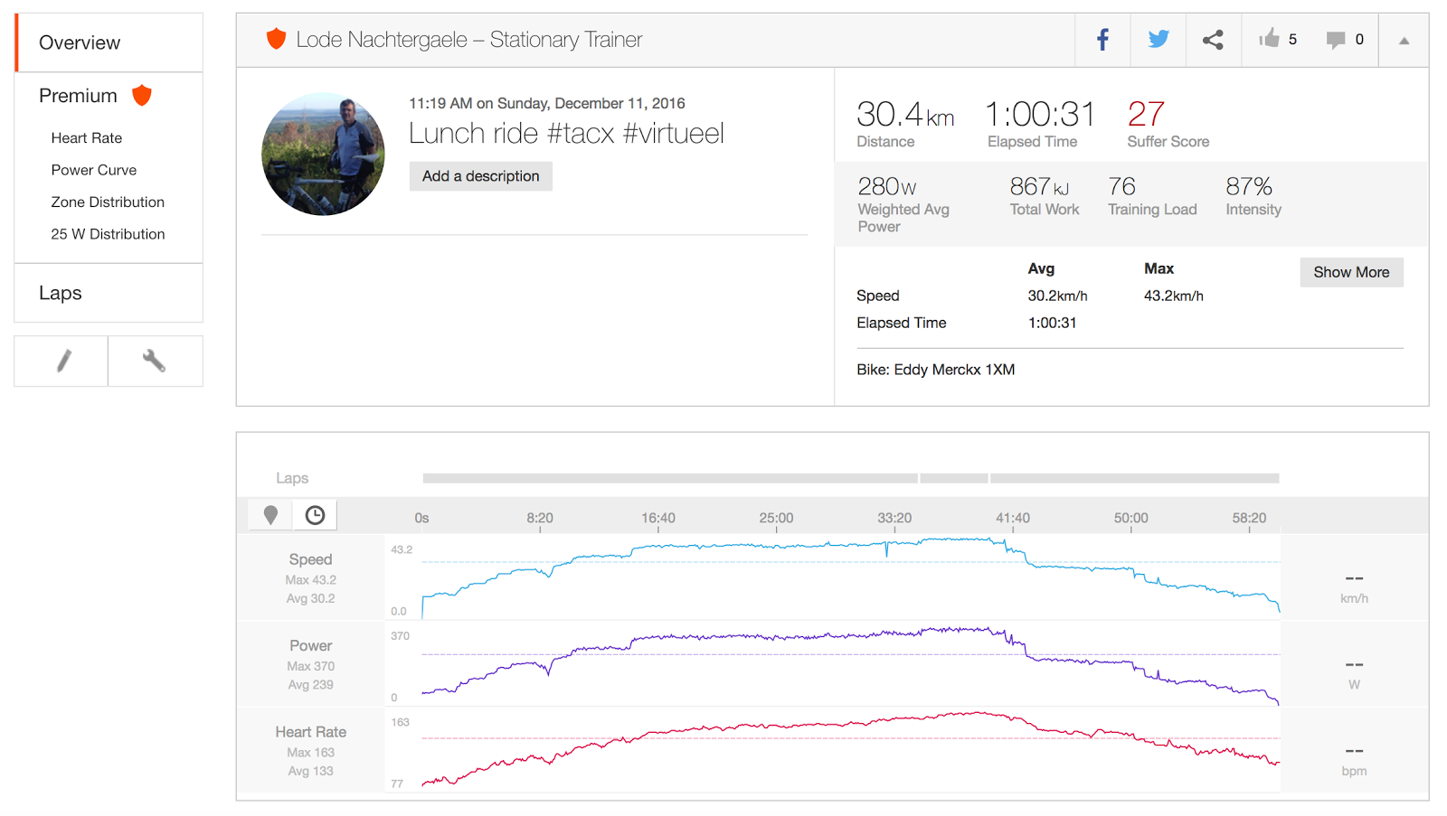
Enter the power meters. They measure exactly what power you're pushing instantaneously. In case of headwind, you'll drive slower but the power readings will be higher. It allows to assess if your body is performing better or not without guessing. Therefore power meters allow to train more scientifically. Power meters give objective values about the performance and hence can be better trusted to evaluate your training efforts.
A central curve helping to gauge your performance is the power duration curve. How many power can you generate for how long ? A typical power curve looks like this:

The horizontal axis is the duration in seconds (usually on a logarithmic scale) and the vertical axis is the delivered power in Watt. The maximum power one can generate for 1 second during a sprint is called the Peak Power. The power one can deliver for one hour is called the Functional Threshold Power (FTP). The limit of the power one can generate forever is called the Critical Power (CP).

But how do we obtain such a curve ? If you record your rides with a computer, software can derive this from the measured values. Since curves of different riders show up similarly, researcher started to believe a model could predict the curve based on some measurements. For example, record how much power you can delivers for 1 minute, 3 minutes and 20 minutes and the whole curve can be reconstructed. In the paper "Rationale and resources for teaching the mathematical modeling of athletic training and performance" by Clarke DC, Skiba PF contains a good overview of the state of the art. The formula to derive power in function of the duration is as follows: $P = AWC (1/t) + CP$ where AWC is the Anaerobic Work Capacity in Joule, $t$ is the duration in seconds and CP is the Critical Power in Watt. The AWC (called W' nowadays) represents the finite amount of energy that is available above the critical power. CP is power that can be sustained without the fatigue for very long time (longer than 10 hours). See also the paper by Charles Dauwe, "Critical Power and Anaerobic Capacity of Grand Cycling Tour Winners".  Recently, @acoggan, @veloclinic and @djconnel are working on more sophisticated models.

@veloclinic proposed in "Cycling Research Study Pre Plan":
$P(t) = \frac{W’_1}{t+\tau_1} + \frac{W’_2}{t+\tau_2}$
and since $W’ = P \times \tau $
$P(t) = \frac{P_1 \tau_1}{t+\tau_1} + \frac{P_2 \tau_2}{t+\tau_2}$
@veloclinic guesses that the new Trainings Peak model to be included in WKO4 is:
$P(t) = \frac{FRC}{t} (1-e^{-\frac{t}{\frac{FRC}{P_{max}-FTP}}}) + FTP + \alpha (t-3600)$
For more information about WKO's new model, watch the youtube video.
And Dan Connelly arrived at:
$P(t) = P_1 \frac{\tau_1}{t}( 1 - e^{-\frac{t}{\tau_1}} ) + \frac{P_2}{(1 + \frac{t}{\tau_2})^ {\alpha_2}}$

Fitting those models to my data, gives the following result (source code):

With some extra code, we can get the confidence interval of the models. For the veloclinic model, the 95% confidence interval is between the dotted green lines (source code):

The estimated veloclinic parameters and their 95% confidence interval are:

• $P_1$ = 291.910642398 Watt [252.385602829  331.435681968]
• $\tau_1$ = 28.6068269179 seconds [17.5113005392  39.7023532965]
• $P_2$ = 800.776804574 Watt [726.249462145  875.304147003]
• $\tau_2$ = 0.312268982434 seconds [-0.16239984039  0.786937805257]

The supposed WKO4 model gives this (source code):

The estimated WKO4 parameters and their 95% confidence interval are:

• FRC = 20463.525586 Joule [13518.0176693  27409.0335028]
• $P_{max}$ = 1011.29658965 Watt [937.344413201  1085.2487661]
• FTP = 257.543501763 Watt [226.388909604  288.698093922]
• $\alpha$ = -0.00512616028401 [-0.00777859140802  -0.00247372916]

And finally, Dan Connelly's model (source code):

The estimated djconnel parameters and their 95% confidence interval are:

• $P_1$ = 730.972437292 Watt, [638.464114912 823.480759673]
• $\tau_1$ = 19.9194404736 seconds [9.71207387339 30.1268070738]
• $P_2$ = 324.66235674 Watt [246.999942142  402.324771339]
• $\tau_2$ = 0.312268982434 seconds [-0.16239984039  0.786937805257]
• $\alpha_2$ = 0.312268982434 [-0.16239984039  0.786937805257]

From those graphs one could derive that the WKO4 model fits best. Remark that this is only the case for my data and that is a too narrow basis to draw such a conclusion. Also my power data itself has to be taken by a grain of salt because I have no power meter and all power data is estimated from other measurements. The dots on the graph are derived from virtual power derived from the speed measurements on my Tacx trainer or by power estimated by Strava on climbs (in that case estimated power by Strava is fairly accurate).

Update: Apparently, the formula in the end of the blogpost from Dan Connely which I used in this blogpost was not correct and must be:
$P(t) = P_1 \frac{\tau_1}{t}( 1 - e^{\frac{-t}{\tau_1}} ) + \frac{P_2}{( 1 + \frac{t}{\alpha_2\tau_2} )^{\alpha_2}}$
Remark the extra $\alpha_2$ in the denomintator under $t$ in the last term of the formula.

Strangely, the confidence interval behaves strange. I have to look into it. The estimated djconnel parameters of the updated model and their 95% confidence interval are:

• $P_1$ = 730.972437292 Watt, [638.464114912 823.480759673]
• $\tau_1$ = 19.9194404736 seconds [9.71207387339 30.1268070738]
• $P_2$ = 324.66235674 Watt [246.999942142  402.324771339]
• $\tau_2$ = 8793.18635004 [-12682.9310423 30269.3037424]
• $\alpha_2$ = 0.312268982434 [-0.16239984039  0.786937805257]

Only the $\tau_2$ parameter changed value, but the confidence interval indicated it does not converge. When starting the optimization function with other initial values, I get overflow errors. To be continued. As Dan remarked we can approximate $\frac{1}{( 1 + \frac{t}{\alpha_2\tau_2} )^{\alpha_2}} \approx (1-\frac{t}{\tau_2 \alpha_2})^{\alpha_2} \approx 1-\frac{t}{\tau_2}$ in the first order. In that case, we get:

The parameters of this simplified model are:

• $P_1$ = 753.75304433 Watt [676.513606926 830.992481733]
• $\tau_1$ = 27.1488626906 seconds [17.4753205281 36.822404853]
• $P_2$ = 275.99764045 Watt [238.468417448 313.526863451]
• $\tau_2$ = 53841.0314734 seconds [30850.1607097 76831.9022372]

Remark that in order to fit the curve the $\tau_2$ parameter must be very big to avoid to get negative power. Hence using the first order approximation is not a good idea.

Another idea I tested is to use a capacity for the second term of Dan Connely's function:

$P(t) = P_1 \frac{\tau_1}{t}( 1 - e^{\frac{-t}{\tau_1}} ) + \frac{P_2 \tau_2}{t+\tau_2}$

This gives the following fitting:

The parameters of this mixed djconel/veloclinic model are:

• $P_1$ = 743.251464989 Watt [666.223087684  820.279842294]
• $\tau_1$ = 23.648384644 seconds [14.5239744624  32.7727948257]
• $P_2$ = 297.690593484 Watt [253.858306164  341.522880804]
• $\tau_2$ = 24294.3750137 seconds [8540.40600978  40048.3440176]

The only thing I hoped to achieve is to offer some software to evaluate power models like those proposed by veloclinic, djconel and acogan. What we now need is a lot of power data so that we can ran those models quickly over that data to draw more solid/general conclusions.

Adding virtual power to TCX for the Tacx Blue Motion Cycling Trainer

I recently bought a cycle trainer for indoor training: Tacx Blue Motion T2600 for 185€ at fiets.be, a local cycling store. Using my Garmin 800, i could record my heartrate, cadence and speed while riding a workout. Since I have no power meter on my bike, I was barred from a feature that higher and more expensive trainers offer. But in the documentation of the trainer, I found a graph showing a linear relation between speed and power. So if I just could add this to the recorded file before submitting it to Strava, I would have trainer for less than 200€ with power measurement. This is the graph:

From that graph we can derive that riding at 60 km/h in position 5 (the middle blue line) a power of 500 Watt is developed. Hence power = speed / 60 * 500 = speed / 6 * 50 . Remark that speed must be in Km/h dimensions to obtain the power in Watt. There's even an interactive graph at website of Tacx. The Garmin 800 measures speed by counting the number of revolution of the wheel in a time unit and multiplying this by the circumference of the wheels. I converted the .fit file, I obtained from the Garmin device, in TCX (a XML file) using Garmin Training Center (Free software available for Windows and Mac). This file basically contains a list of trackpoints (1 trackpoint every second). One trackpoint looks like this:

        <Trackpoint>
            <Time>2014-01-29T20:38:59Z</Time>
            <AltitudeMeters>157.4000244</AltitudeMeters>
            <DistanceMeters>14850.7099609</DistanceMeters>
            <HeartRateBpm xsi:type="HeartRateInBeatsPerMinute_t">
              <Value>139</Value>
            </HeartRateBpm>
            <Cadence>92</Cadence>
            <Extensions>
              <TPX xmlns="http://www.garmin.com/xmlschemas/ActivityExtension/v2" CadenceSensor="Bike">
                <Speed>8.4530001</Speed>
              </TPX>
            </Extensions>
          </Trackpoint>

At this time, the speed was 8.4530001 meter per second. To convert this to km/h, we have to divide by thousand and multiply by 3600 (the number of seconds in an hour). So speed_in_kmperh = speed /1000.0 * 60 *60 = 30.43080036 km/h. The power developed at that moment was : 30.43080036/6.0*50.0 = 253.590003 Watts. We convert to integer : 253 Watt. To add this to the TCX file, we add a line <Watts>253</Watts> as follows:

        <Trackpoint>
            <Time>2014-01-29T20:38:59Z</Time>
            <AltitudeMeters>157.4000244</AltitudeMeters>
            <DistanceMeters>14850.7099609</DistanceMeters>
            <HeartRateBpm xsi:type="HeartRateInBeatsPerMinute_t">
              <Value>139</Value>
            </HeartRateBpm>
            <Cadence>92</Cadence>
            <Extensions>
              <TPX xmlns="http://www.garmin.com/xmlschemas/ActivityExtension/v2" CadenceSensor="Bike">
                <Speed>8.4530001</Speed>
                <Watts>253</Watts>
              </TPX>
            </Extensions>
          </Trackpoint>

The next step was to automate the calculation of the power and adding it to the TCX file. I wrote the following Python script to do that:

prompt> python vpower.py > vpower_29-01-14\ 20-53-27.tcx

I uploaded the resulting TCX file to Strava and obtained this:

Of course, the power in this workout is based on the fact that I left the lever om my trainer on position 5 during the whole workout. If you change the position of the lever during the workout, this approach will give wrong results.

Is this approach of "virtual power" accurate ? Not as accurate as power meters on the bike but usable I would argue. The concept of "virtual power" is also supported by Trainer Road Software. Later, I found an interactive graph of the speed power relation for Tacx Blue Motion on the website of Tacx. From that graph, I could obtain more precise datapoints : at 60 km/h power is 407 Watt. So next time I use my script, I will use power = speed_in_kmperh / 60.0 * 407.0 as power formula.